Introduction
A goal for this post is to convert the dataset to a dataframe for analysis and performing a regression on the state.x77 dataset.
Results
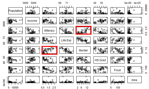
Figure 1: Scatter plot matrix of the dataframe state.x77. The red box illustrates the relationship that is personally identified for further analysis.


Figure 2: Scatter plot of murder rates versus illiteracy rates across the united states, with the linear regression function of illiteracy = 0.11607 * Murder + 0.31362; with a correlation of 0.729752.
Discussion
This post analyzes the dataset state.x77 under the MASS R library, was converted into a data frame (see code section), and an analysis of the data was conducted. To identify which variable relationship would be interesting to conduct a regression on this dataset, all the relationships within the data frame were plotted in a matrix (Figure 1). The relationship that personally seemed interesting was the relationship between illiteracy and murder. Thus, moving forward with these variables a simple linear regression was conducted on that data. It was determined that there is a positive correlation on this data of 0.729752, and the relationship between the data is defined by
illiteracy = 0.11607 * Murder + 0.31362 (1)
From this equation that describes the relationship (Figure 2) between these variables, can explain, 53.25% of the variance between these variables. Both the intercept value and the regression weight are statistically significant at the 0.01 level, meaning that there is less than a 1% chance that this relationship could be developed from pure random chance (R output between Figure 1 & 2). In conclusion, this data is stating that states with lower illiteracy rates will have the least amount of murder rates in their state, and vice versa.
Code
#
## Converting a dataset to a dataframe for analysis.
#
library(MASS) # Activate the MASS library
library(nutshell) # Activate the nutshell library to access the plot function
data() # Lists all data and datasets within the Mass Library
data(state) # Data in question is located in state
head(state.x77) # Print out the top five entries of state.x77
df= data.frame(state.x77) # Convert the state.x77 data into a dataframe
#
## Regression formulation
#
plot(df) # Scatter plot matrix, of all relationships between the variables in the df
stateRegression = lm(Illiteracy~Murder, data= df) # Selecting this relationship for further analysis
summary(stateRegression) # Plotting a summary of the regression data
# Plotting a scatterplot from a dataframe below
plot(df$Murder, df$Illiteracy, type=”p”, main=”Illiteracy rates vs Murder rates”, xlab=”Murder”, ylab=”Illiteracy”) # Plotting a scatterplot from a dataframe
abline(lm(Illiteracy~Murder, data= df), col=”red”) # Plotting a red regression line
cor(df$Murder, df$Illiteracy)
References
- Berkeley Statistics (n.d.). Data Frames and Plotting. Retrieved from http://www.stat.berkeley.edu/~s133/R-4a.html
- Dalgaard, P. (2011). [R] state.x77 dataset. Retrieved from https://stat.ethz.ch/pipermail/r-help/2011-March/271280.html
- Marin, M. (2013) Linear regression in R (R tutorial 5.1). Retrieved from https://www.youtube.com/watch?v=66z_MRwtFJM
- R (n.d.). Plot Method for Data Frames. Retrieved from https://stat.ethz.ch/R-manual/R-devel/library/graphics/html/plot.dataframe.html
- R (n.d.). Return the first or last part of an object. Retrieved from https://stat.ethz.ch/R-manual/R-devel/library/utils/html/head.html
- Schumacker, R. E. (2014) Learning statistics using R. California, SAGE Publications, Inc, VitalBook file.
